How to convert a distance matrix to a pairwise table with R
This page shows how to export a distance matrix from UGENE, then use the R statistical software to convert the text file from a square matrix into pairwise columns suitable for other work.
- Export/save matrix as a space-delimited text file for use as an R data file
- Start R and after loading the data file
- Run some script using reshape package
What we want is to convert from the matrix to a column. Thus, from a matrix (Table 1)
Table 1. Hamming distances among three taxa for cytochrome c protein
| Human | Alligator | Fish | |
| Human | 0 | 13 | 20 |
| Alligator | 13 | 0 | 19 |
| Fish | 20 | 19 | 0 |
to a pairwise column (Table 2)
Table 2. Pairwise comparisons
| Pair | Distance |
| Human – Alligator | 13 |
| Human – Fish | 20 |
| Alligator – Fish | 19 |
The distances then could be plotted against divergence time (human – alligator: 320 mya, human – fish: 432 mya, alligator – fish: 432 mya) for a molecular clock analysis (Fig 1)

Figure 1. Scatter plot of Hamming distance by divergence times.
We’ll outline the steps from alignment of sequences to computing a distance matrix in UGENE.
From sequences to distances
Assuming you have a list of accession numbers for your sequence, then open UGENE and create a New Project. This example we use cytochrome c protein sequences obtained by BLASTp.
Table 3. Accession numbers used in this exercise
| taxa | accession number |
| Human |
NP_061820.1 |
| Alligator |
KYO26818.1 |
| Fish |
P81459.1 |
To load accession files into UGENE, navigate to File → Access remote database…, then copy/paste the accession list to UGENE (Fig. 2).

Figure 2. Fetch (add) accessions to UGENE project.
Assuming all is well, you’ll see sequence files added to your project, one at a time (Fig. 3).
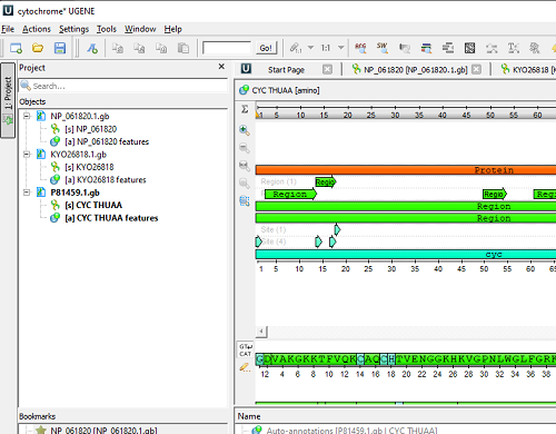
Figure 3. Sequence files added to UGENE project.
After loading the sequences, conduct a multisequence alignment, e.g., MUSCLE. Once this has completed, right-click in the Alignment window and select from the context menu: Statistics → Generate distance matrix… (Fig. 4)

Figure 4. Selecting distance matrix export from UGENE alignment window context menu
Next, choose the distance algorithm (default – Hamming dissimilarity), exclude gaps, Save profile to file, select correct folder to save the file, and select Comma separated (CSV) (Fig. 5). Create a filename, e.g., CYCS_distance_matrix.csv.
Select “Generate” when ready.
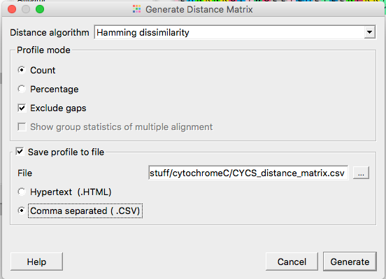
Figure 5. Options in UGENE to specify distance matrix output.
You have in your hands a text file containing a square distance matrix, like this one (Fig 6).
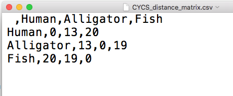
Figure 6. Screenshot of the CSV text file from within TextEdit on macOS.
Take a moment to verify that Figure 6 and Table 1 are the same.
From matrix to columns
We are ready to proceed to convert the matrix to a pairwise column. For a simple matrix like this, it is probably just as quick to do it by hand. This option rapidly loses its appeal as the matrix gets larger. For example, with just 14 taxa, there are 92 pairwise comparisons to make!
We assume that you have a working copy of R installed on your computer. If not, see Install R at Mike’s Biostatistics Book.
Start R.
Point R to your working directory, the one that contains your matrix file. Our example, the file name was CYCS_distance_matrix.csv. In R script, replace filename.txt with the name of your matrix csv file.
R script
At the R prompt run each line one at a time (red text after “#” are comments, ignored by R. You don’t have to copy the comments)
getwd() ................................#check working directory
setwd("/pathname") .............#change working directory to "/pathname"
my_data <- read.table("filename.txt", header=TRUE)
my_data...............................#this will print out your table so you can inspect it
library(reshape)...................#this package has useful functions for reworking your data table
m <- as.matrix(my_data)
m2 <- melt(m)[melt(upper.tri(m))$value,]......#this transposes the upper triangle of your table into three columns: a column from the header row, the first column containing the species names and then the third contains the distances
names(m2) <- c("spp1", "spp2", "distance")......#this adds header row
m2......................................#this will print out your table so you can inspect it
write.csv(m2, file = "outfile.csv").......#this will save your file as a csv text file
/MD