Tree reconciliation
Note: This is a long page with 17 images.
Work to do: update links
What you need to do this exercise
You need
- rooted gene tree file. If you have not rooted your gene tree, do so now. Follow instructions at Change root for gene tree.
- copy of the Newick code for our consensus tree. This available on this page as Tree14 (with branch lengths) and Tree14NO (without branch lengths. It is also available at An example consensus phylogenetic tree.
What software to use
Option 1. Use R software and associated packages. Click here
Option 2. Use CompPhy, a web app. Click here
Background
The apply the molecular clock model of evolution to our gene tree of the 14 taxa in order to estimate the rate of evolutionary change. The primary assumption is that the rate of molecular evolution (specifically, the rate of amino acid substitutions) is roughly constant over time and across different lineages. In this exercise we provide the first of two ways to test whether or not this assumption holds for our gene trees: tree reconciliation. The other option, Tajima’s rate test, is provided at Evolutionary rate tests.
Slides to support this text and brief how to video with CompPhy and Unipro UGENE. The slide show lacks narration.
Evolution is change in the heritable characteristics of biological populations over successive generations. Speciation, from one interbreeding population to two separate populations, leads to lineages isolated from each other. Isolation here means that the two populations do not exchange genes, and, therefore, changes over generations that occur in the sequence of a gene in one species, whether by genetic drift or natural selection, are independent of changes that may have occurred in the sister species.
The forces* that create genetic variation (mutation, recombination) and filter genetic variation (natural selection, genetic drift) in populations may occur at the same rates in the two distinct lineages, but by no means is this assumption likely to be true for all genes or DNA elements. For example, if one population undergoes a bottleneck, a severe reduction in population size, then this population would see significant reduction in genetic variation because of random genetic drift on the kinds of alleles present in the population.
*Note: The use of the term “force” is an analogy, not to be confused with the forces of Newtonian mechanics.
Tree reconciliation, whereby a gene tree is compared to a species consensus phylogeny (Page 1994; Jackson 2005), is an approach to estimate or highlight any inconsistencies between genes, and the the evolutionary histories of species (Maddison 1997). In brief, you count the number of nodes in common between the two trees. The more in common, the greater the similarity, the more the gene tree reflects what we believe is the true phylogeny. To the extent the trees do not agree, this tells us that any number of artifacts (e.g., long-branch attraction, poor sequence alignment, paralogs and not orthologs used), or evolutionary events (incomplete lineage assorting, unequal rates of evolution) may apply to our gene tree. To the extent that our gene trees disagree with the consensus tree, this weakens the use of the Molecular Clock model to evaluate our genes.
How many nodes in a gene tree with k = 14 species (tips)? It’s helpful to distinguish between internal nodes (ancestors) and tip nodes (the taxa in the study). For a strictly bifurcating tree (no polytomies), there will be k – 1 internal nodes and k tip nodes. Thus, total number of nodes is 2k – 1. Thus, for our 14 species problem there are 27 nodes. Similarly, the number of branches is 2k – 2 — except for the root node, all nodes have three connecting branches: a branch connecting with the ancestor and two branches connecting each of the descendent nodes, therefore, 26 branches for k = 14.
Our consensus phylogeny, Tree14, is shown in Fig. 1A (with Newick string in Fig 1B). Where the trees differ, the gene tree is said to be discordant, also called incomplete lineage sorting. Tree discordance will be evidenced by odd groupings in the gene tree, e.g., Alligator and Pig, Fig. 2A). Possible evolutionary explanations include gene rate of evolution (e.g., long branch attraction), gene duplication, or horizontal gene transfer. Long branch attraction is a type of systematic error: two distantly related taxa have the same sequence, not because of shared recent ancestry, but because mutation space has saturated. More simply, there are limited number of possible changes (only the four nucleotide bases, only 20 amino acids), a gene that is rapidly evolving will show spurious (not valid) similarity. Thus, the longer the time since divergence, the sequences will be “attracted to each other,” hiding true phylogenetic relationships (Baldauf 2003).
Reconcile and test assumption of equal rates
We can compare the gene tree against the phylogeny. How much in agreement are the two trees? We can consider two ways
1. Obtain similarity of the tree topology by applying one of the many tools available
- the statistical programming language R (
apeandphytoolspackages installed)- extensive notes are provided; even if you choose not to use R, you should skim through to pick up pointers on how to interpret tree reconciliation results.
- Click here to go to Use R option
- CompPhy, an online site that will compare trees
- Update Spring 2022 — this is probably your best option
- Click here to go to Use CompPhy option
2. Test the hypothesis that evolutionary rates are the same
- compare agreement of nodes with a binomial test
- conduct a rate test of amino acid substitutions
1. Obtain similarity of trees
Given a calibrated phylogeny for the taxa, gene trees can be compared against the “true” phylogeny (i.e., our consensus tree), and amount of agreement can be scored. Comparing phylogenies is a remarkably vibrant field, with new approaches, from visualization to statistical tests, appearing in the literature each year. Thus, we will use a variety of approaches.
You generated a consensus phylogeny for our 14 species from data at NCBI Taxonomy (Lab 5: Phylogenetics). Note that although we intended to take this as a our consensus tree, you should try the set of dichotomous branches linking the 14 taxa (e.g., shown in Fig 1A, also provided at Our consensus phylogeny), because your NCBI consensus tree had several polytomies (three or more tops connected to a node). Therefore, I recommend you first compare your gene tree against a completely bifurcating phylogeny as the consensus phylogeny, like the the one shown in Figure 1A (Newick code for the tree displayed in Figure 1B, see also Our consensus phylogeny;).
What follows next is a worked example. You may also follow along by using the DOCK2 gene tree I provide here (Fig. 2A and 2B); for your own project you would use your gene tree and compare against the consensus tree (Fig 1A and 1B).
Example data
Figure 1A shows your consensus phylogeny, tree14, generated from timetree.org.
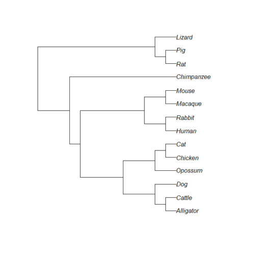
Figure 1A. Consensus phylogeny, tree14, for our 14 species, compiled from data available at timetree.org. Branch lengths not displayed. Newick text in Figure 1B.
((Lizard:279.65697667,(Chicken:236.50266286,Alligator:236.50266286):43.15431381):32.24694470,(Opossum,(((Cat:54.32144118,Dog:54.32144118):23.43351523,(Cattle:61.96598852,Pig:61.96598852):15.78896789):18.70743276,((Rabbit:82.14079889,(Rat:20.88741740,Mouse:20.88741740):61.25338149):7.68238853,(Macaque:29.44154682,(Chimpanzee:6.65090500,Human:6.65090500):22.79064182):60.38164060):6.63920175):62.13519841):153.30633379);
Figure 1B. Newick code for consensus phylogeny, tree14, displayed in Figure 1A.
And for our example, a Maximum Likelihood gene (DOCK2) tree (rooted) was constructed for the same taxa (Anolis = Lizard, Cattle replaces Cow) and is shown in Figure 2A, with Newick file in Figure 2B. Of course, replace my example tree with your GOI/protein tree for your project.
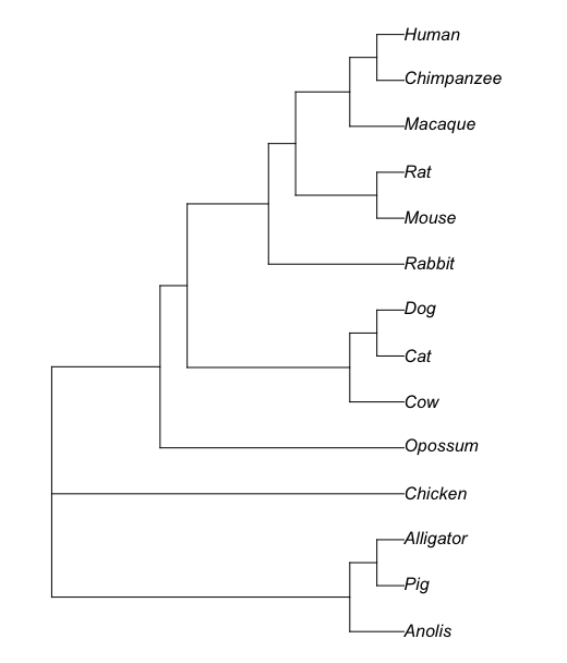
Figure 2A. DOCK2 gene tree, rooted. Branch lengths not displayed. Note Anolis = Lizard, Cow = Cattle.
((Lizard:0.108121,(Pig:0.537039,Alligator:100)0.11963:0.581483)1.98059:0.0219903,Chicken:0.080801,(Opossum:0.0317054,((Cattle:0.0431675,(Cat:0.00979658,Dog:0.0087833)44.5528:0.00810975)6.61867:0.00465613,(Rabbit:0.0237457,((Mouse:0.013629,Rat:0.0260838)306.257:0.0301612,(Macaque:0.00405341,(Chimpanzee:0.00115417,Human:0.00115316)22.9446:0.00249574)90.1845:0.0107642)18.4444:0.00497191)14.5323:0.00414756)137.68:0.035267)384.224:0.0835984);
Figure 2B. Newick code for tree in Figure 2A. Note: Changed Anolis to Lizard, Cow = Cattle.
Note: While UGENE has some capabilities to manipulate and display trees (rooting, swapping nodes), the ape and phytools packages for R statistical software language have a lot more features. I have included scripts for each step discussed. I’ve also provided alternatives to using R, compPhy and phylo.io, which can do some of the work
Option 1. Use of R
Start your analysis with Data management — remove the branch lengths from your Newick files
The branch lengths in the consensus tree (Fig 1A and 1B) are divergence times in millions of years (mya), and are not comparable to the branch lengths, which are genetic distances, in my gene tree example(Fig. 2A and 2B). You’ll need to remove the branch lengths before trying the reconciliation steps.
Like all data management operations, you can choose a method that works best for you. One choice — simply load the tree file into your text editor and delete by hand each of the “:nnnn” branch (actually, they are called edges in bioinformatics-speak). (For help with text editors, see Text files are data files.)
For example, before editing we have
((Lizard:279.65697667,(Chicken…
After editing you would have
((Lizard,(Chicken…
Editing by hand will work, provided you are careful and don’t miss details. For my gene tree example, more than 30 separate edits are required! Seems risky, too many opportunities for error.
Thus, a far better option is to use an application to automatically edit, don’t you think? So, consider learning how to use R, a statistical programming language. You have three options for using R.
- Install R onto your computer.
- While in the end this is the better option, be aware that this route will take you much longer to complete today’s exercise. There’s a significant learning curve for working with R.
- As an alternative, you can take advantage of rdrr.io, which allows you to run small amounts of R code online.
- Another option — You may want to explore using Jupyter Notebooks, which allow you to mix R code snippets with other text or graphs (in other words, a nice way to do bioinformatics! A way to combine your code methods with results for your lab notebook).
Let’s discuss the second option first. You can run small amounts of code at https://rdrr.io/snippets/ (or from the homepage, click on “Run R code online”), or even from this page (scroll to the bottom, or click here, and you’ll find an embedded R snippet). Simply copy/paste or enter your commands in the box, replacing the example code there. An example of one of our code snippets is shown in Fig 3.
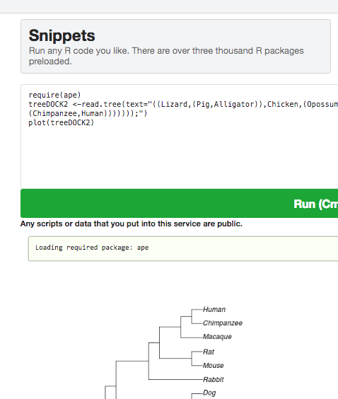
Figure 3. Screenshot from rdrr.io with R code snippet.
The first option is the best option: go ahead and get for yourself an up-to-date copy of R installed on your computer. Once you install R on your own computer, you’ll also need to download and install two additional packages, ape and phytools.
Regardless of the option you choose, proceed by copy/paste the code I provide below, one line at a time at the R prompt. For , or better, create a script file (from the R GUI, File → New document). Run each command one a time: simply hit the Enter key to submit the command; if using a script file, then Ctrl+R for windows PC, Command + Enter for macOS.
R Code example: Remove branch lengths
Those of you working with a local installation of R (or R and RStudio), create an R script file and copy/paste code from our web site to the script file. For rdrr.io users, copy/paste the code into the text box available at the website.
R works line by line; lines that begin with # are ignored by R and are provided as comments or notes about the code. Text in blue represents the code you enter; text in red represents the output R provides in response to the commands.
The following code is used to strip the branch lengths from our consensus tree Newick file, shown in Fg 2B.
require(ape)
require(phytools)
#Copy the Newick data, in this case, topology only
tree14 <-read.tree(text="((Lizard:279.65697667,(Chicken:236.50266286,Alligator:236.50266286):43.15431381):32.24694470,(Opossum,(((Cat:54.32144118,Dog:54.32144118):23.43351523,(Cow:61.96598852,Pig:61.96598852):15.78896789):18.70743276,((Rabbit:82.14079889,(Rat:20.88741740,Mouse:20.88741740):61.25338149):7.68238853,(Macaque:29.44154682,(Chimpanzee:6.65090500,Human:6.65090500):22.79064182):60.38164060):6.63920175):62.13519841):153.30633379);")
plot(tree14)

#Strip branch lengths, h/t Liam Revell
tree14NO <- tree14
tree14NO$edge.length<-NULL
write.tree(tree14NO)
After submitting the write.tree() command, R returns with what we want.
[1] "((Lizard,(Chicken,Alligator)),(Opossum,(((Cat,Dog),(Cow,Pig)),((Rabbit,(Rat,Mouse)),(Macaque,(Chimpanzee,Human))))));"
I would then use tree14NO, not tree 14 for comparisons. And you should too. In other words, just copy the output above and add to your R code
tree14NO <- read.tree(text="((Lizard,(Chicken,Alligator)),(Opossum,(((Cat,Dog),(Cattle,Pig)),((Rabbit,(Rat,Mouse)),(Macaque,(Chimpanzee,Human))))));")
Figure 2B. Newick file for DOCK2 gene tree, View in icyTree
R code example for our gene tree. Again, replace with your Newick code for your own gene tree, as appropriate. If you are running a local installation of R, you do not need to repeatedly load ape and phytools libraries. If you are using rdrr.io, you will, of course, need to load the libraries for each iteration.
#Note that I removed branch lengths to compare topology only
treeDOCK2 <-read.tree(text="((Lizard,(Pig,Alligator)),Chicken,(Opossum,((Cattle,(Cat,Dog)),(Rabbit,((Mouse,Rat),(Macaque,(Chimpanzee,Human)))))));")
plot(treeDOCK2)
Note: For those of you with R or RStudio installed on your computer, you should have R extract your Newick code directly from the file saved on your computer. For example, we’ll assume your working directory is BI308L located on your Desktop. You’ll want to set R’s working directory to the folder in which the Newick file is stored. To check current working directory used by your session of R, use the getwd() command.
getwd()
On my computer, R returns
[1] "/Users/mikedohm/Desktop/BI311"
We want BI308L, so
setwd("/Users/mikedohm/Desktop/BI308L")
will do the job. Confirm by invoking the getwd() command.
Now, when we wish to load a Newick string into an R session, instead of copying and pasting the Newick string from a text file between the “” in the text= portion of the command
read.tree(text="")
we simply type in the name of the Newick file, replacing text= with file=
read.tree(file="tree14.nwk")
Pause for a moment
Remember the scientific purpose for this lab exercise, which is to test for agreement between your gene tree and the consensus phylogeny. Discrepancies between your gene tree and the consensus phylogeny tell you about the evolutionary history of your gene, and, therefore, about whether or not variation in the human gene is likely to be due to random chance or natural selection.
If you are getting impatient, skip past this section to get instructions compPhy. The next sections do contain more than just instructions with R; there are mentions of how to interpret the results of node counting, which should be read by all.
Do the trees agree? Visuals first
Before proceeding, please review what product you are expected to generate to complete this lab exercise.
Reconciliation analysis involves comparing two related phylogenies. The particular way we compare two trees is cophylogeny mapping (Page 1994, Jackson 2005). The next series of instructions all accomplish the same task: to compare the topologies of the two trees. I’ll present script examples you can run in R, plus instructions for CompPhy and phlo.io, two online tools that can be used to compare trees to obtain graphics and/or count the differences between the gene and consensus phylogenetic trees.
R code examples — display tree discordance
Our first approach is simply to plot the trees in a way that we can compare them visually. A crude estimate is to match the branch nodes in common between the two trees (Figure 3A, R script in Figure 3B).
Visualization 1
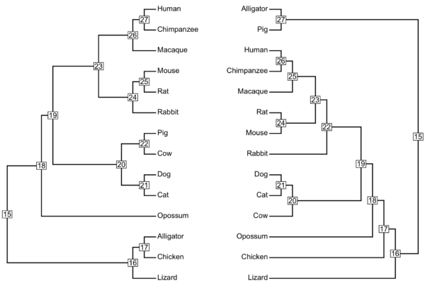
Figure 4. The same trees from Fig 1A and Fig 2A, but with nodes labeled. The consensus tree is shown at left, the gene tree is shown on the right.
R code to make the Fig 4 plot.
#set plot device to one row, two columns
par(mfrow=c(1,2))
#you may beed to stretch the window that pops up -- sometimes the plots disappear if you don't open up a larger window
plotTree(tree14NO,node.numbers=TRUE)
plotTree(treeDOCK2,direction="leftwards",node.numbers=TRUE)
#dev.off resets the plot device specified by par()
dev.off()
Figure 4 is pretty hard to look at and count the differences.
Part of the problem with this approach is that we confuse how the topology is ordered vertically in our graphic visualization for actual differences in the tree shape (topology). While the topology (branching) is not arbitrary, how the pairs of taxa are displayed is arbitrary. For example, find the rat/mouse clade in Figure 4. There’s nothing to infer that in the left-hand figure, mouse is top and rat is bottom — note that in the right-hand plot, rat is on top and mouse is bottom. Thus, while Visualization 1 meets the criteria, to compare the gene tree against the consensus tree, the visual doesn’t really help the reader compare the trees!
We’ll need to rotate the tips to better align the tree where we can. We’ll present more sophisticated methods below, see Visualization 2.
It’s OK to go ahead and just count the matches by hand, but a starter would be to run a simple script in R
#If not already done so, load the libraries
require(ape)
require(phytools)
#Code starts here
all.equal(tree14NO, treeDOCK2)
If the two trees had the same branching order, then this function would return TRUE. In our case, the results were
[1] FALSE
Not very informative. Try matchNodes(tree1, tree2, c("descendants")
matchNodes(tree14,treeDOCK2,c("descendants"))
#R returns with
=> Comparing tree14 with treeDOCK2.
Both trees have the same number of tips: 14.
Both trees have the same tip labels.
Both trees have the same number of nodes: 13.
Both trees are rooted.
Both trees are not ultrametric.
7 clades in tree14 not in treeDOCK2.
7 clades in treeDOCK2 not in tree14.
The matchNodes() command assumes we have already rotated the trees, and thus is does not allow us to rotate the trees with this function, so we’ll keep going. We could go back to our tree drawing software like UGENE or icyTree and accomplish the rotations of the trees individually to match them up as best we can, but the point of our journey is to introduce you to program/software solutions. Lets keep going.
A note about “ultrametric.” An ultrametric tree is one in which all the branch lengths, from root to tips, are the same length. This would be consistent with a perfect molecular clock in which rates of evolution are the same for all lineages. UPGMA algorithm is one of the oldest clustering algorithms, creates ultrametric trees.
Visualization 2.
A more sophisticated version of the graph we just try is available with the comparePhylo() command (ape package)
comparePhylo(tree14NO,treeDOCK2, plot=TRUE)
Results from comparePhylo() include the same output from matchNodes, plus a graph (Fig. 5).
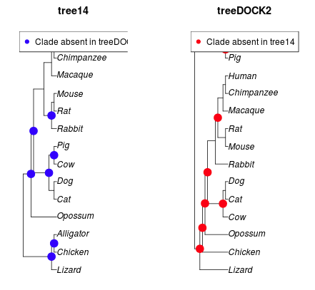
Figure 5. A graphic from comparePhylo() function call, R package ape. Note that I haven’t figured out how to fix the label problems!
comparePhylo() is like matchNodes: also does not allow us to try and rotate the tree. Keep going
And here’s a “tanglegram” (Fig. 6). A tanglegram can be used to reflect topology differences between two trees. At last! Options to rotate. I’ll post both the unrotated and the rotated graphs. We’ll compare how many nodes actually differ between the gene tree and the consensus phylogeny.
With the R code to make the tanglegram, adapted from Liam Revell’s example, our first run does not rotate the trees.
tangleTree<-cophylo(tree14NO,treeDOCK2,rotate=FALSE)
plot(tangleTree)
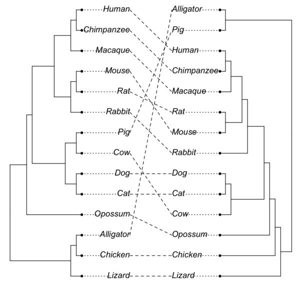
Figure 6. A tanglegram for the same trees, no rotation. Command tangelgram, cophylo(), rotate=FALSE.
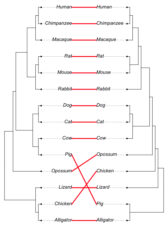
And our example with rotation (Fig. 7). I’ve included multi.rotate=TRUE.
Note. You could also just use rotate=TRUE instead of multi.rotate, provided there are no polytomies in either tree.
tangleTreeRotate<-cophylo(tree14,treeDOCK2,rotate.multi=TRUE)
plot(tangleTreeRotate,link.lwd=3,link.lty="solid", link.col=("red"),fsize=1)
 +
+
Figure 7. The tanglegram, now with rotate=TRUE.
At last, we have our answer! How many nodes differ? Three nodes.
Get distance measure between the two trees
After obtaining a suitable visual, calculate measures of distance between the two trees. You’ll need an additional R package called phangorn.
require(ape)
#require(phytools)
require (phangorn)
#Code starts here
tree14NO <- read.tree(text="((Lizard,(Chicken,Alligator)),(Opossum,(((Cat,Dog),(Cow,Pig)),((Rabbit,(Rat,Mouse)),(Macaque,(Chimpanzee,Human))))));")
treeDOCK2 <-read.tree(text="((Lizard,(Pig,Alligator)),Chicken,(Opossum,((Cow,(Cat,Dog)),(Rabbit,((Mouse,Rat),(Macaque,(Chimpanzee,Human)))))));")
treedist(tree14NO, treeDOCK2,check.labels = TRUE)
and the results from R are
RF.dist(tree14NO, treeDOCK2, normalize = FALSE, check.labels = TRUE, rooted = FALSE)
results should be the same as symmetric.distance (also called Robinson-Foulds metric), 12
SPR.dist(tree14NO, treeDOCK2)
For these two trees, the minimum number of SPR moves to convert the trees was 3. SPR moves refers to “Subtree Prune and Regraft,”
Option 2. Use of CompPhy
A better statistic is to calculate a measure of how dissimilar the two trees are. Link to CompPhy by Fiorini et al (2014), which can be used to calculate the symmetrical distance RF between the two trees. The algorithm is an implementation of Felsenstein’s treedist from the package PHYLIP (Fiorini et al. 2014). The greater the score for the symmetrical distance, the more different the two trees are from each other.
Using CompPhy is straightforward, but may take you a couple of attempts to get the results.
- You can register or work anonymously. It is definitely best if your register (it’s free!).
- The consensus tree and your gene tree must be saved to individual files. CompPhy does not have a copy/paste option.
- Click on New Project to begin; if you register, then you can find saved projects in My project in the menu bar at top.
- Enter a project title and project description.
- Check the format for Newick and drag each phylogeny file to the first (left) window (Tree collection 1). Note in this example I loaded both trees into Collection 1, then ignored Collection 2. ; both of your trees go to Collection 1. You may have to enter a project name for Collection 2 — do so, then proceed
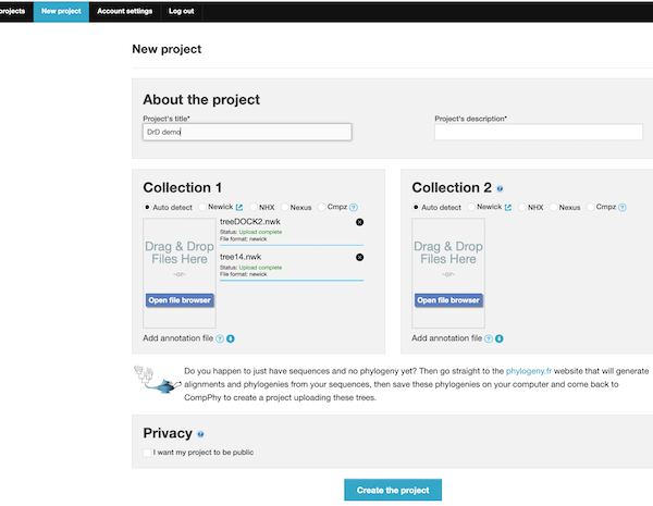
Figure 8. Screenshot setup New project at CompPhy. Note two Newick files
- Once the trees are loaded, drag each to a window (screenshot in Figure 9).
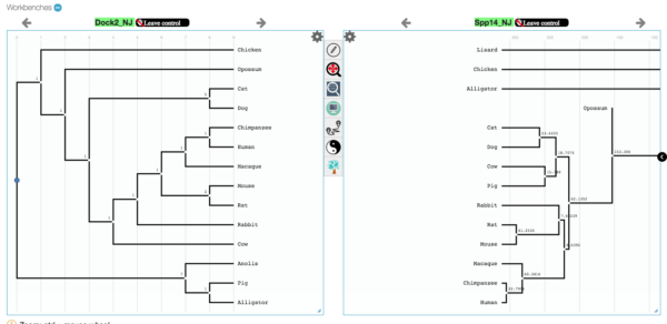
Figure 9. Screenshot, trees loaded in CompPhy workbench
- After creating a project and loading trees, you can add trees later via the upload option (Fig. 10). Scroll down to end of Project page for Miscellaneous tools.
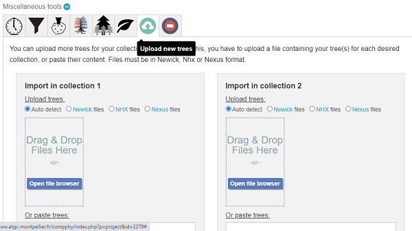
Figure 10. Screenshot, miscellaneous tools, upload additional trees to your CompPhy project
- Run the program — you may have to wait a while for the program to complete comparisons of the two trees.
- Once both trees are in memory, you can click on the Symmetry RF button (Fig 11, magnified view Fig 9) to obtain the estimate of the symmetrical distance statistic.
![]()
Figure 11. Isolated and magnified view of Symmetry RF button in CompPhy (see Fig 9). Click this button to obtain the symmetry (dissimilarity) value of the trees.
Results
For the two trees shown in Figure 2 (and again in Figure 6), the similarity score was ten (Fig 12).
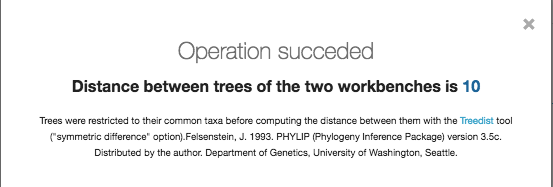
Figure 12. Screenshot, output from CompPhy for similarity RF score.
Interpretation?
In general, the lower the score the more similar the trees are. For DOCK2 we got 10; for another gene, OLFML2B we got 12. Thus, the DOCK2 gene tree was more in agreement to the consensus phylogeny than was OLFML2B gene tree. Once I receive reconciliation results from the class, I will collate all of your results into a table available to you after spring break, which will allow you to compare your gene against the others for a sense of how different your gene is.
2. Test the hypothesis.
We’ve generated a number of ways of visualizing how well our gene trees match our consensus phylogeny. We can do more than visualize, we can make statistical tests. After all, a few differences doesn’t seem like much disagreement, but as the number of differences between our trees grow, at some point it seems like a big difference. Taking a statistical approach allows us to quantify what we mean by a difference. We’ll try a simple approach. For a rooted tree there are tips minus one numbers of internal nodes. For our tips = 14, then, there are 14 – 1 = 13 internal nodes. We can count up the matches between the two trees and compare the observed matches against the expected with a binomial.
![]()
where p is the probability of success (branch nodes match) and n is the number of trials (nodes), and X is the number of observed matching nodes. For example, from Figure 7 we counted matches of 10 out of possible 13 nodes. A crude estimate of how often we would expect a match by chance would simply be 1 divided by 13 = 0.077, which we’ll take as p, our probability of success. How likely is a match of 10 if by chance alone?
Here’s the R code
dbinom(10, 13, 0.077)
and the result
Alternatively, you could use your spreadsheet application (Google Sheets, LibreOffice Calc, Microsoft Excel, even Apple’s Numbers, although not as easy), and enter the function call in any empty cell
=BINOM.DIST(10,13,0.077,0)
(The zero at the end tells your spreadsheet that you want the individual probability calculated, not the cumulative.)
The result is the same: the p value is very, very small. The number of observed successes (node matches) between the DOCK2 gene tree and the consensus phylogeny was 10. Thus, probability of getting this many matches and the two trees by chance alone are the same was P = 1.65 x 10⁻⁹, which is much (much!) smaller than 5% (our typical “is it significant?” statistical cut-off), we conclude that the gene tree matches our consensus phylogeny.
References and further reading
Baldauf, S. L. (2003). Phylogeny for the faint of heart: a tutorial. TRENDS in Genetics, 19(6), 345-351. (link)
Castresana, J. (2007). Topological variation in single-gene phylogenetic trees. Genome biology, 8(6), 216. (link)
Fiorini, N., Lefort, V., Chevenet, F., Berry, V., & Chifolleau, A. M. A. (2014). CompPhy: a web-based collaborative platform for comparing phylogenies. BMC evolutionary biology, 14(1), 253. (link)
Jackson, A. P. (2005). The effect of paralogous lineages on the application of reconciliation analysis by cophylogeny mapping. Systematic biology, 54(1), 127-145. (link)
Kendall, M., & Colijn, C. (2016). Mapping phylogenetic trees to reveal distinct patterns of evolution. Molecular biology and evolution, 33(10), 2735-2743. (link)
Maddison, W. P. (1997) Gene trees in species trees. Systematic Biology 46(3):523-536.
Page, R. D. (1994). Maps between trees and cladistic analysis of historical associations among genes, organisms, and areas. Systematic Biology, 43(1), 58-77.
Tajima, F. (1993). Simple methods for testing the molecular evolutionary clock hypothesis. Genetics, 135(2), 599-607. (link)
Vaughan, T. G. (2017). IcyTree: Rapid browser-based visualization for phylogenetic trees and networks. Bioinformatics , 33(15), 2392-2394. DOI: 10.1093/bioinformatics/btx155
Run your R code!
Copy and paste R code here. Edit as needed.
/MD