Sequence alignment: Basics explained
Page work to do
fix images- fix links
- add menu
- remove CANVAS remarks
The purpose of this lab is to
- Learn how to load files into UGENE, perform basic tasks like sequence alignment and viewing sequences and their annotations.
- Learn about gap penalty and weight matrix usage
- Extract basic statistical summaries like a grid profile to summarize results from the alignment
- Next week, Construct trees: Building the gene tree — The basics explained and Make a gene tree
Can’t wait to start?
Scroll down the page to What to do: The alignment
Background
Sequence Alignment
- The process or result of matching up the nucleotide or amino acid residues of two or more biological sequences to achieve maximal levels of identity and, in the case of amino acid sequences, conservation, for the purpose of assessing the degree of similarity and the possibility of homology.
A basic question about any biological sequence is to ask if it is related to any known sequence, a sequence deposited and available in one of the public databases. In biology, homology means shared features as a result of descent from a common ancestor. Similarity may also mean the two proteins have similar function.
Thus, in biology, similarity of two protein sequences suggests that they are homologous. We can distinguish two kinds of homology: ortholog sequences, where the two sequences owe their similarity to descent from a recent, common ancestor, and parolog sequences, where the two sequences owe their similarity because of convergent evolution, not recency of shared ancestry.
When considering sequence alignment, where the multiple sequences share the same nucleotide at the same position in the DNA sequence, we expect the algorithms to find such matches. As the length of the matches increase, our confidence in the alignment also increases. Where the algorithms differ is how they work with differences among the sequences. We can distinguish between base substitutions, transitions (purines to purines, i.e., A ↔ G, or pyrimidine to pyrimidine, i.e., C ↔ T), transversions (purine to pyrimidine or ), and indels (insertion or deletion). For proteins, likelihood of amino acid substitutions
Consider an SNP [G/A] at a particular location in the genome (a transition base substitution). Two individuals (taxa) may share the SNP because they are orthologous, or because they are paralogous. The two kinds of homology are illustrated in Figure 1A (ortholog) and Fig. 1B (paralog).
![Example of orthologs. The two taxa share the [G/A] transition because they shared a common ancestor.](https://geneticslab.letgen.org/wp-content/uploads/2025/03/orthologSNP-e1742076773190.png)
Figure 1A. Example of orthologs. The two taxa share the [G/A] transition because they shared a common ancestor.
![Example of paralogs. The two taxa independently evolved the [G/A] transition.](https://geneticslab.letgen.org/wp-content/uploads/2025/03/paralogSNP-e1742076846470.png)
Figure 1B. Example of paralogs. The two taxa independently evolved the [G/A] transition.
Note that the process of establishing alignment among biological sequences from organisms is linked to hypotheses of the evolutionary relationships (i.e., phylogeny) among those organisms. In essence, the fact that sequences can be aligned is taken as evidence for the homology of those sequences. Now, understand that establishing homology between two species requires more than simply aligning sequences, requiring analyses that include outgroups. You should be asking why two events in Figure 1B and not just a single reversion from A → G? One, we know that G → A is more common than A → G (because C spontaneously deaminates to U, then leads to C → T transition; then on the complementary strand you will have G → A). For another reason, we would conduct such analyses by comparing against an outgroup (Fig 2).
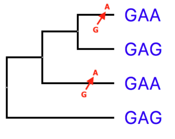
Figure 2. An outgroup allows you to determine likely ancestral states of characters.
But for our purposes, this is the intent of constructing and evaluating alignments among sequences: to establish homology of those sequences.
Algorithms
We will work primarily with the alignment software Clustal Omega. Clustal Omega is descended from Clustal W perhaps the most widely used local alignment tool, and does an adequate job. It is not necessarily the best tool in part because its underlying algorithm has not been updated since the 1990’s (Bradley et al 2009). CLUSTALW however remains relevant in part because it is widely used, but also for pedagogical purposes because it permits us to introduce the idea that sequence alignment has as its core, assumptions about evolutionary processes. Additionally, CLUSTALW serves well to introduce the problems inherent in adding “biology” to the bioinformatics.
CLUSTALW uses a progressive approach to solve multiple sequence alignment problems: an initial pairing of two sequences is done, followed by pairing of the next sequence to the consensus sequence of the first pair, and so on until all comparisons have been made. Because errors in the initial pairwise comparison carry over to later alignments, the progressive alignment approach is expected to have some difficulty with distantly related sequences.
T-COFFEE is a variant of CLUSTALW and, while slower, is thought to do a better job at alignment than CLUSTALW. UGENE provides a GUI for CLUSTALW, T-COFFEE, and other alignment applications, in which the user selects from a variety of options to guide the alignment process.
More recent research efforts utilize “hidden Markov models” abbreviated as HMM. Clustal Omega uses HMM. Markov models are stochastic (random) probability models that are used to make predictions about events. For example, Brownian motion can be modeled by one class of these stochastic models (see this great animation of Brownian motion at Wikipedia). Markov models are based on the Markov property — future events depend only on the present, not on the sequence of events that led to the present position. In “simple” Markov models, going from one position (state) to another is visible so the transition probabilities can be estimated; in hidden Markov models, the initial state is not known, but the outcome state is observable, so the transition probabilities from one state to another take a different format.
See Pais et al (2014) for more details and comparisons of the algorithms.
Substitution matrices (PAM and BLOSUM)
Aligning sequences, whether it is DNA or protein sequences, requires a model for how change is expected to occur. One approach is to view change in sequence as a Markov Chain process. For the DNA example, the states are {A, C, G, T]; for the protein example, the states are the {20 amino acids}. Some math follows to calculate the transition probabilities, the chance that an “A” changes to a “T” (etc.). Jukes-Cantor is one attempt at modeling these transition probabilities, it makes the assumption that all kinds of substitutions are equally likely to occur. This is, of course, counter to our observations: For DNA, transition probabilities (purine to purine, or pyrimidine to pyrimidine) are likely different that transversion probabilities (purine to pyrimidine or vice versa). For proteins, the basic idea follows, but with 20 instead of four states, and therefore, many more transition probabilities need to be assigned. Whatever the model, the goal then is to use the model to assist in the alignment procedure. More realistic models provide better alignment, but at cost of computation speed (or may not be solvable at all). A compromise is usually made where a scoring matrix is constructed so that, based on the assumptions and model of substitution probabilities, some alignments are given higher scores than others.
Considering the problems with multiple sequence protein alignment, scoring matrix may give higher scores in alignments where identical amino acids are aligned, higher scores when conservative substitutions (e.g., amino acids with similar chemical characteristics), and even some weight given to homology considerations (e.g., if comparing mouse with rat, as opposed to mouse and yeast). PAM and BLOSUM are scoring matrices for protein alignments. PAM (stands for “Accepted Point Mutation”) invokes a Markov process and was built from observations of closely related species. Accepted mutations were those that were commonly observed and therefore did not adversely affect the protein function. They began with species that were judged to be closely related, inferred the ancestral sequence, and aligned the sequences for a protein. From the presumed ancestral species, counts of the number of replacements were taken. These counts were used to calculate the Markov transition probabilities. PAM therefore incorporates known phylogeny into the equation. PAM1 refers to the rate of substitution if 1% of the amino acids had changed. Additional PAM matrices are calculated from the 1% PAM with the assumption that more change would in sequence would follow the basic pattern established for more distantly related sequences. PAM30 and PAM70, representing 30% and 70% expected change are the generally used scoring matrices for this approach. (Click here to see the PAM30 matrix values; click here for the PAM70 mat
[under construction — see Wikipedia for more details] BLOSUM (BLOcks SUbstitution Matrix) is another substitution matrix used for sequence alignment of proteins. BLOSUM matrices are used to score alignments between evolutionarily divergent protein sequences (Henikoff and Henikoff). All BLOSUM matrices are based on observed alignments; they are not extrapolated from comparisons of closely related proteins like the PAM Matrices.
Why do sequences of the same gene (DNA element) diverge?
DNA and therefore protein sequences differ among species because the (1) sequences diverged since the last common ancestor of these species or (2) prior to speciation, there was duplication of the gene and, by errors in replication, the gene copies diverged. Consider that mice, chickens, alligators, Xenopus frogs, and humans all have a gene for hemoglobin subunit beta. How similar are these species for hemoglobin? I used BLASTp to find the accession numbers for this protein for each of the listed species. I then used our UGENE to collect and align the sequences. (Click here for the protocol.) I then constructed a gene (phylogenetic) tree three ways: Neighbor Joining (NJ, Fig 3), Maximum Likelihood (ML, Fig 4), and Bayesian (MrB, Fig 5). UGENE uses a mid-tree rooting, which is an arbitrary setting of the putative ancestral node. UGENE allows you to reset the root, or, in the case of these figures, I used a better tree drawing program called FigTree to set the root correctly (icyTree.org is a great online tool for displaying trees, but as of this writing, it can’t set root).

Figure 3. Here is the Neighbor-Joining tree. Branch lengths shown
Maximum likelihood tree (Fig. 4)

Figure 4. Maximum likelihood tree, which constrains branch lengths so that negative lengths are not possible.
And last, the Bayesian tree (Fig 5).

Figure 5. The Bayesian tree of the same hemoglobin sequences.
Note that these gene trees are very similar: chicken and alligator form a clade (as they should); mouse and human form a clade according to Bayes and ML approach, again, as we would expect; and the Xenopus frog form the outgroup (as expected). With just five taxa it’s hard to separate these trees, but either the Bayes or ML trees would be better choice than the NJ tree, which failed to assign the mouse and human sequences.
We distinguish between two kinds of alignment: global and local. Global alignment implies that the sequences are optimally aligned across the entire sequence. Local alignment, in contrast, infers that alignment has been done for a portion of the sequence. BLAST is a local alignment tool, we are using progressive multiple sequence alignments based on local alignments.
Analysis of relatedness is accomplished by aligning sequences. Homology of two sequences may be extensive or it may be partial: sequences may share domains or motifs.
Software to run and view alignment
UniPro UGENE
Online: https://alignmentviewer.org/ : load MSA FASTA format
https://www.jalview.org/
What to do: The alignment
See help files
After loading your 14 accession numbers into UGENE (see Introduction help pages!), after exporting the sequences to the alignment window, right-click in the alignment window to bring up the menu (Fig 5.)
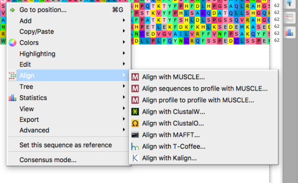
Figure 5. Screenshot UGENE app (macOS). Right-click in alignment window to bring-up the menu, select Align to bring up the alignment algorithms available.
Try as your default choice ClustalO, then try T-Coffee. Remember that you can’t simply run T-Coffee alignment on the aligned sequences from ClustalO. Rather, go back select the sequences from the Project window, export them again, then run alignment with T-Coffee algorithm. Save as different alignment files.
For each, obtain basic statistics about the alignments (available by clicking on the “bar graph icon tab, Fig. 6).
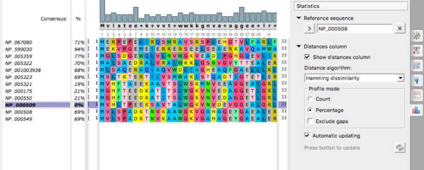
Figure 6. Screenshot UGENE app (macOS). Gather statistics for the sequences, e.g., calculate Hamming distance.
Take one sequence as the reference, then compare the Hamming distances for each sequence. Hamming distance is simply the number of differences, n, between two aligned sequences of length N. The distance is then n/N, usually represented as a percentage. For example, Table 1 shows results for alignments of human globin genes.
Table 1. Hamming distance calculated from alignments by ClustalO, T-Coffee, and MUSCLE. Myoglobin (+MB) taken as reference sequence.
| Protein | ClustalO | T-Coffee | MUSCLE |
| HBA1 | 69% | 71% | 64% |
| HBA2 | 69% | 94% | 79% |
| HBB | 77% | 77% | 62% |
| HBG1 | 77% | 70% | 50% |
| HBG2 | 76% | 68% | 52% |
| HBE1 | 76% | 69% | 51% |
| HBZ | 71% | 19% | 19% |
| HBM | 78% | 21% | 20% |
| HBQ1 | 72% | 21% | 21% |
| MB | 0% | 0% | 0% |
| CYGB | 92% | 69% | 46% |
| NGB | 73% | 69% | 46% |
How to know which alignment is “best”?
Protein sequence alignment for multiple species is the first step for many analyses, including (from Nute et al. 2018):
- detection of natural selection
- predicting ancestral protein sequences
- predicting protein function
- protein domain identification
- protein-protein interactions
Thus, it follows that finding the best alignment for all included sequences is important step. What constitutes “best?” Over the years, researchers have accumulated sequences for many members of protein families; generating alignments of these families has led to a series of benchmarks (e.g., Bahr et al 2001). Comparing our sequence alignments against these benchmarks is a way for us to make a qualitative judgement about whether or not our alignments are the best possible.
Another approach employs statistical approaches that incorporate phylogenetic trees and evolutionary models of change. UGENE does not have this capability, but we can find access to a software implementation of one such efforts, called PRANK (no, I’m not kidding), from the European Molecular Biology Laboratory – European Bioinformatics Institute at https://www.ebi.ac.uk/goldman-srv/webprank/, and an older version (but with more output options), at https://www.ebi.ac.uk/Tools/msa/prank/
So, how well did our collection of algorithms in UGENE do against these more sophisticated options? I used PRANK on the same set of sequences for human globins. Briefly, from within UGENE, export the sequences for alignment, select FASTA format. Then load the FASTA file into the PRANK page and submit the file to run the analysis. After a few minutes, results are returned (Fig open browser to
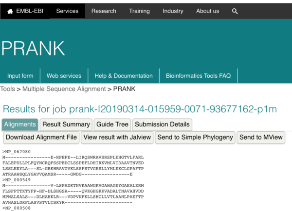
Figure 7. Screenshot. Results window from the PRANK program at EMBL-EBI.
Finally, download the alignment file (FASTA format), then load into UGENE. Note that if your browser is like mine, it will want to add a .txt extension. Change to .fa extension for FASTA format. UGENE will respond better for you.
How did we do? I calculated Hamming distances for the PRANK results, now added to our comparisons of the algorithms (Table 2).
Table 2. Added results for PRANK. Correlation calculated for each method with results from PRANK.
| Protein | ClustalO | T-Coffee | MUSCLE | PRANK |
| HBA1 | 69% | 71% | 64% | 59% |
| HBA2 | 69% | 94% | 79% | 59% |
| HBB | 77% | 77% | 62% | 60% |
| HBG1 | 77% | 70% | 50% | 60% |
| HBG2 | 76% | 68% | 52% | 60% |
| HBE1 | 76% | 69% | 51% | 61% |
| HBZ | 71% | 19% | 19% | 59% |
| HBM | 78% | 21% | 20% | 60% |
| HBQ1 | 72% | 21% | 21% | 61% |
| MB | 0% | 0% | 0% | 0% |
| CYGB | 92% | 69% | 46% | 73% |
| NGB | 73% | 69% | 46% | 67% |
| correlation | 98% | 58% | 56% |
We would conclude from this that Clustal Omega did the best — or at least agrees with PRANK.
Product progress
The Report 2 project will have several steps. For each step, you’ll want to create PowerPoint files to capture what you’ve done. By the end of the semester, the report is completed by merging (and editing as needed) all slides of the project steps and adding your conclusions.
You do not have to upload any slides from this day’s work — but they will be part of your Report 2.
This step, Align Brief.
Slides to include for your Report 2:
- Alignment by ClustalO
- Alignment by T-Coffee
- Table comparing %differences by the two alignment methods
Pay attention to filename conventions for your project.
Once you have what you believe is the best alignment, proceed to making your gene tree.
Week 5: Make a tree
Once you have established alignments for your protein sequences, construct three trees:
- Neighbor Joining tree
- Bayesian tree
- Maximum likelihood tree
Next: Lab 5: Phylogenetics and Lab 5: Make a gene tree
What about the trees? Don’t turn them in now, just the alignment results. We will work on these throughout the week; they will be turned in as part of next week’s lab
Questions
References
Bahr, A., Thompson, J. D., Thierry, J. C., & Poch, O. (2001). BAliBASE (Benchmark Alignment dataBASE): enhancements for repeats, transmembrane sequences and circular permutations. Nucleic Acids Research, 29(1), 323-326. https://dx.doi.org/10.1093%2Fnar%2F29.1.323
Bradley RK, Roberts A, Smoot M, Juvekar S, Do J, et al. (2009) Fast Statistical Alignment. PLoS Comput Biol 5(5): e1000392. https://doi.org/10.1093/nar/29.1.323
Blair, C., & Murphy, R. W. (2011). Recent trends in molecular phylogenetic analysis: where to next? Journal of Heredity, 102(1), 130-138. https://doi.org/10.1093/jhered/esq092
Bykova, N. A., Favorov, A. V., & Mironov, A. A. (2013). Hidden Markov models for evolution and comparative genomics analysis. PloS one, 8(6), e65012. link
Chatzou, M., Magis, C., Chang, J. M., Kemena, C., Bussotti, G., Erb, I., & Notredame, C. (2016). Multiple sequence alignment modeling: methods and applications. Briefings in bioinformatics , 17 (6), 1009-1023. doi.org/10.1093/bib/bbv099
Nute, M., Saleh, E., & Warnow, T. (2018). Evaluating Statistical Multiple Sequence Alignment in Comparison to Other Alignment Methods on Protein Data Sets. Systematic biology.
Pagel, M., Meade, A., & Barker, D. (2004). Bayesian estimation of ancestral character states on phylogenies. Systematic biology, 53(5), 673-684. link
Pais, F. S. M., de Cássia Ruy, P., Oliveira, G., & Coimbra, R. S. (2014). Assessing the efficiency of multiple sequence alignment programs. Algorithms for Molecular Biology, 9(1), 4. doi:10.1186/1748-7188-9-4
/MD