Make a gene tree

to do:

• update links
• add workflow image
• menu, split pages

The purpose of this lab is to

1. Construct a NJ tree
2. Construct ML tree (use PhyML or IQ-TREE)
3. Construct Bayesian tree
4. Next Lab: Gene Tree/Phylogeny reconciliation and rates:

Overview of the project

You construct a gene (protein) tree, working with the gene product (protein) from your PheGenI project Report 2: Bioinformatics project — Overview. By now, you will have conducted multiple sequence alignments for fourteen homologous (orthologs) protein sequences, including the human gene of interest sequence identified by you from the PheGenI database Lab 2: PhenGenI Brief. By now, you’ve acquired your accessions and aligned the sequences. You are ready to construct a gene tree. You should also review Phylogenetics before beginning your work.

Background

We’ve talked about phylogeny already, see Phylogenetics. Species trees reflect the history and divergence of species, gene trees represent the evolutionary history of the gene itself. Differences between the two can occur because of

1. Gene duplication. A gene duplicates into two paralogs within an ancestral genome. If one copy is lost in one lineage and the other copy is lost in another, the remaining genes will appear to violate the species tree topology (Goodman et al 1979).
2. Gene loss: Following duplication or polyploidy, one of the copies may be lost (pseudogenization), leading to misinterpretation of orthology (Goodman et al 1979, Xiong et al 2022).
   • “Pseudogenization” (Jacq et al 1977 cf. discussion in Podlaha and Zhang 2010), refers to process of a functional gene changes to nonfunctional pseudogene due to the accumulation of mutations.
3. Incomplete lineage assortment — where ancestral polymorphisms are retained through rapid speciation events and sort independently into the daughter species — can cause gene trees and species trees to diverge (Davidson et al 2015 and references therein).
4. Rapid, differential rates of gene evolution among lineages can also lead to gene-species tree discordance by causing long-branch attraction.
   • Long branches, representing high amounts of molecular change, are mistaken for shared, derived characteristics (homoplasy).

Reminder: orthologs – homologous genes originating via speciation (matching the species tree) rather than paralogs, whereby homologous gene copies arise by duplication within the same lieage.

Here, we present briefly information about how gene trees are made, the algorithms and the assumptions. As explained in class, I am asking you to submit just one tree, made by the Maximum Likelihood approach. However, you are expected to create gene trees using all three methods in order to make comparisons about which algorithm performed best (i.e., which method recreated the expected species phylogeny). We discuss analyses for tree reconciliation — the process of embedding gene tree within the species tree– at Tree reconciliation (Goodman et al 1979; Swenson and El-Mabrouk 2012). Rate tests (Tajima 1983) are introduced at Evolutionary rate tests.

Neighbor Joining approach

Neighbor Joining (NJ) is a statistical tool for clustering (grouping) objects for which distances have been obtained. The distances between each pair of objects (e.g., taxa) are arranged in a matrix. The NJ algorithm them joins groups of objects by the distances between them, linking groups of objects with short distances and distributing other such groups that have greater distances between them. The algorithm does this repeatedly, joining all of the groups until a statistical criterion is reached. This criterion is a “minimum evolution” requirement, which means that the resulting tree has branch lengths as short as they can be.

Among all of the approaches to tree-building, NJ is a very fast method and it has the property that if the distance matrix is correct (i.e., accurately reflects the true evolutionary story among the taxa included), then the NJ method will return a tree that accurately reflects that story. In other words, the branching patterns will be correct. NJ may be the only reasonable choice if working on a large data set, In general, it is not considered the best algorithm choice.

NJ was introduced in 1987 (Saito and Nei, 1987), and remains a useful tool to this day;  distance methods have largely fallen out of favor, replaced by ML and Bayesian approaches. NJ is very fast, and is used to construct guide trees for MJ and Bayesian phylogeny software

Maximum Likelihood approach.

UGENE includes PhyML, or Phylogenetic Analysis using Maximum Likelihood analysis of protein and DNA sequences. Guindon et al 2009, Guindon et al 2010.

Maximum likelihood is a statistical method to estimate the parameters of a statistical model, given the set of observations. Given the amino acid (or nucleotide) differences among aligned sequences (i.e., the set of observations), what model maximizes the likelihood of the data? PhyML gives the approximate probability that a particular branch exists in the true phylogenetic tree.  Uses sophisticated models that specify substitution (e.g., LG), gamma distribution (normal distribution is an example of a gamma distribution). Although computationally intense It has repeatedly been demonstrated that these models are able to recover the true tree or a tree which is topologically closer to the true tree more frequently than less elaborate methods such as parsimony or neighbor joining.

Bayesian approach.

In phylogenetics based on biological sequences for a set of organisms, Bayesian analysis refers to a statistical approach to data inference (hypothesis testing); the researcher holds a model of the evolution for a set of taxa and then the software searches for the set of phylogenetic trees that are consistent with the model and the alignment data. The model of relationships is based on our prior knowledge; the goal of the Bayesian approach is to see if new information improves the fit of the data to the model.

Bayesian analysis seeks the tree that maximizes the probability given both the model and the data. In Bayesian terminology, this probability is the posterior probability, or our confidence in the model given the fit to the data; the model is viewed as the prior probability.

The basis for Bayesian approach: Given a prior probability(e.g., our model of evolution among the species), calculate the posterior probability of the new tree. The prior probability can be thought as follows: we know a bunch about evolution (captured by models we choose), we know a bunch about how species are related to each other (fossil evidence, results from other gene trees yield a consensus tree), therefore, it makes sense to incorporate prior knowledge and weigh new data against this understanding. Then, each tree calculated gets a posterior probability associated with it; as the software compares the various trees calculated, then the higher the posterior probability, the greater the likelihood the tree is the correct one.

Bayesian analyses returns a set of best trees, with statistical support for each branch length. MrBayes, available in UGENE, implements Bayesian approach to phylogeny construction (Huelsenbeck and Ronquist 2001).

Do the work → Document fully in your Lab Notebook

Once you have established alignments for your orthologous protein sequences, construct your three gene trees. In general, accept the default settings, with the exception that you’ll want to click on Display option tab and check the box (Fig. 1) so that your trees are displayed in a new window, not, as default, alongside the alignments (the view gets very crowded on laptop screens).

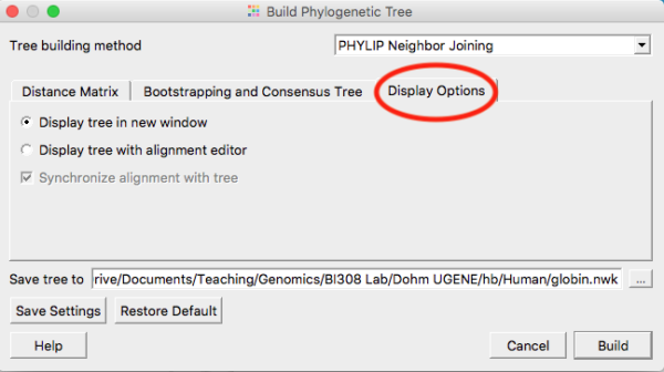
Figure 1. Select the Display option tab (shown in screenshot with red circle) and choose Display tree in new window

Note: Once you have changed the setting to Display tree in new window, click on the “Save settings” button. UGENE will remember your preference and next time you won’t have to make this change.

First, start with the NJ tree.

Start in the alignment window, right-click in alignment window to bring-up the menu, select Tree (Fig 2), then Build tree to bring up the tree algorithms available (Fig 3-5).

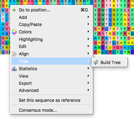
Figure 2. Right-click in alignment window to bring-up the menu, select Tree, then Build Tree, to bring up the tree algorithms available.

Neighbor joining is the default selection. At least for now, don’t adjust any of the defaults. We will discuss in class these selections and what they mean. Do click on “Display options” tab and select to Display the tree in its own window.  For now, just click “Build” button to proceed (Fig 3).

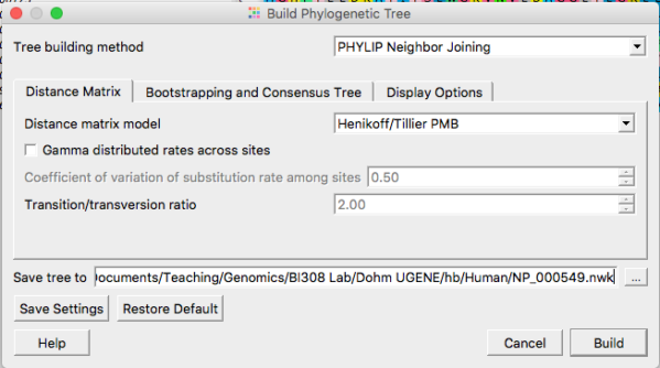
Figure 3. Options for Neighbor Joining algorithm include choosing types of distances calculated and assumptions about mutations. 

The NJ approach is very fast so you’ll have results right away. Do take the time to inspect the topology and branch lengths. After changing from the default mid-rooting to a proper outgroup root, NJ approaches can yield negative branch lengths between tips, which is, of course, biologically impossible. Negative branch lengths may be improved upon by returning to and paying more attention to the sequence alignments Refining and improving alignments. If you are unable to improve the alignment sufficient to eliminate negative branch lengths, open your Newick file in a text editor and replace the negative branch lengths with a value of 0 (zero).

And again, you are expected to document choices you make in your Lab Notebook.

Oops. You forgot to uncheck the Display tree option, now you have a screen that looks like Figure 4 — both alignment window and the tree window crowded together on your screen in one tab. Here’s how to fix this.

Click on the >> in the Tree view portion of the tab. This brings up a menu (Fig 5).

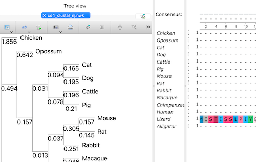
Figure 4. Screenshot of Unipro UGENE with both alignment and tree in same, crowded view.

Select Disable Tree and Alignment synchronization (Fig 5), then try closing one of the tabs.

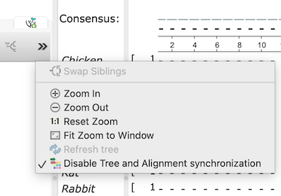
Figure 5. Screenshot of Unipro UGENE sub-menu. Select Disable Tree and Alignment synchronization.

Second, after obtaining your NJ tree, make an ML tree.

For a number of reasons, maximum likelihood (ML) trees (and Bayesian algorithms) are better — more accurate — than NJ trees (discussion and references in Ruriko and Masatoshi 2016). Go ahead and grab the ML tree (Fig 6). The app is called PhyML (IQTREE is also available, and often, but not always leads to higher ML ). Again, for now, accept the default settings. Expect to wait a few minutes before the tree building is complete. In the newest version of UGENE (ver 41), a new maximum likelihood app called IQ-TREE is now available. It should be much faster than PhyML. You may use either one — just be clear which you are running. Accept default suggestions, make note that this was your choice in your notebook.

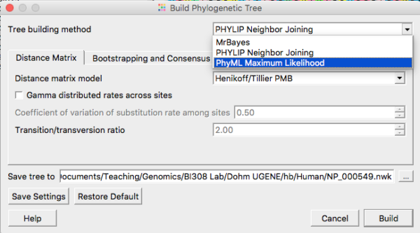
Figure 6. Select Maximum Likelihood routine from the Tree Build menu.

And last, make the Bayesian tree

See Figure 7 to select MrBayes tree building options. Accept defaults. Bayesian algorithms, like ML algorithms are much slower than the NJ approach — expect to wait a few minutes before the tree building is complete.

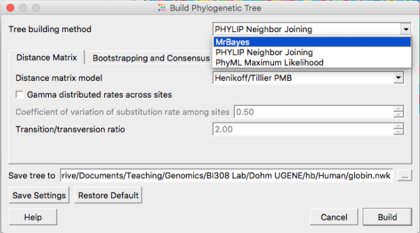
Figure 7. Select MrBayes routine from the Tree Build menu.

Note that you saved the tree file to your folder selected in the Save tree to dialog box (Fig. 5).

Now done with all three, compare

In your lab notebook, conclude this exercise by making observations and comparisons among the resulting trees. Which pairings are consistent among all three trees? Other observations? I’m looking for you to describe what you see. Optionally, you can make a more complete comparison among your three gene trees by exploiting techniques discussed in Working with gene tree: Reconciliation and Working with gene tree: Rate tests.

Product to turn in

At the end of this exercise, please submit all three trees (Neighbor Joining, Bayesian, Maximum Likelihood); paste the Newick file to Submit Newick file here 

The simplest thing to do is to open each tree file (e.g., in example, globin.nwk) in your favorite text editor, then copy/paste in the text box where you submit your Newick file in CANVAS.

Note1: Where’s your Newick files? You saved your UGENE project files to your working directory, correct? Alternatively, in UGENE Objects pane, scroll down to find your Newick file(s), then right-click on the filename and select Open containing folder. This opens Explorer (WinPC) or Finder (macOS) and you can then select your Newick files.

Note2: Remember, you can’t just click on your Newick file in Explorer or Finder. Your operating system associates file extensions with apps, and the .nwk extension is likely associated with UGENE. So, just right-click on the file then select Open with and choose your editor, either Notepad (WinPC) or TextEdit (macOS).

The Report 2 project will have several steps. For each step, you submit PowerPoint files. By the end of the semester, the report is completed by merging (and editing as needed) all of the project steps.

This step does not require you to turn in any product. However, you are encouraged to make appropriate PowerPoint (saved as pdf) files for use in your Final Product

Questions

Week 6 questions Quiz: Trees and Newick files

References

Blair C, Murphy RW Recent trends in molecular phylogenetic analysis: where to next? J Jered 2011 102(1):130-138.

Davidson, R., Vachaspati, P., Mirarab, S., & Warnow, T. (2015). Phylogenomic species tree estimation in the presence of incomplete lineage sorting and horizontal gene transfer. BMC genomics, 16(Suppl 10), S1.

Felsenstein, J. (1981). Evolutionary trees from DNA sequences: a maximum likelihood approach. Journal of molecular evolution, 17(6), 368-376. link

Goodman M, Czelusniak J, Moore G, Romero-Herrera A, Matsuda G. Fitting the gene lineage into its species lineage, a parsimony strategy illustrated by cladograms constructed from globin sequences. Systematic Zoology. 1979;28:132–163.

Graham, C. H., Storch, D., & Machac, A. (2018). Phylogenetic scale in ecology and evolution. Global Ecology and Biogeography, 27(2), 175-187. DOI: 10.1111/geb.12686

Guindon, S., Delsuc, F., Dufayard, J. F., & Gascuel, O. (2009). Estimating maximum likelihood phylogenies with PhyML. In Bioinformatics for DNA sequence analysis (pp. 113-137). Humana Press. (Link to manuscript, pdf)

Guindon, S., Dufayard, J. F., Lefort, V., Anisimova, M., Hordijk, W., & Gascuel, O. (2010). New algorithms and methods to estimate maximum-likelihood phylogenies: assessing the performance of PhyML 3.0. Systematic biology, 59(3), 307-321. (link to website)

Huelsenbeck, J. P., & Rannala, B. (1997). Phylogenetic methods come of age: testing hypotheses in an evolutionary context. Science, 276(5310), 227-232. link)

Huelsenbeck, J. P., and F. Ronquist. 2001. MrBayes: Bayesian inference of phylogenetic trees. Bioinformatics 17:754-755. https://doi.org/10.1093/bioinformatics/17.8.754

Liò, P., & Goldman, N. (1998). Models of molecular evolution and phylogeny. Genome research, 8(12), 1233-1244.  link

Podlaha, O., & Zhang, J. (2010). Pseudogenes and their evolution. Encyclopedia of life sciences (ELS), 1-8.

Saitou, N., & Nei, M. (1987). The neighbor-joining method: a new method for reconstructing phylogenetic trees. Molecular biology and evolution, 4(4), 406-425. link

Schliep, K. P. (2010). phangorn: phylogenetic analysis in R. Bioinformatics, 27(4), 592-593.

Swenson, K. M., & El-Mabrouk, N. (2012). Gene trees and species trees: irreconcilable differences. BMC bioinformatics, 13(Suppl 19), S15.

Warren, D. L., Geneva, A. J., & Lanfear, R. (2017). RWTY (R We There Yet): an R package for examining convergence of Bayesian phylogenetic analyses. Molecular Biology and Evolution, 34(4), 1016-1020.

Xiong, Haifeng, Danying Wang, Chen Shao, Xuchen Yang, Jialin Yang, Tao Ma, Charles C. Davis, Liang Liu, and Zhenxiang Xi. (2022). Species tree estimation and the impact of gene loss following whole-genome duplication. Systematic Biology 71(6) : 1348-1361.

/MD