Cell counts by spectrophotometer
draft
Approximate counts by spectrophotometer
If cells are grown in suspension, eg, bacteria, yeast, or Schneider cells, then if light is passed through the suspension, the amount of light passed through the suspension will be inversely related to the concentration of the cells in the suspension. An “absorbance” reading at 600 nm is used and original suspension may need to be diluted to keep within the limits of the spectrophotometer. Optical density (OD) readings between 0.1 and 0.7 are optimal — above an OD of 1.0 and 90% or more of the transmitted light is scattered, noticeable nonlinear.
This technique relies on light scattering, turbidity, not light absorption, and the Beer-Lambert law does not strictly apply to scattering in dense suspensions. Whereas absorption suggests light is absorbed by molecules within the solution, changing energy states, cells in suspended solution scatter light, which reduces detector intensity. Light scattering is proportional to cell concentration over a narrow range. True absorbance follows the Beer-Lambert law, making scattering better for microbial growth monitoring and absorbance better for molecular quantification. What is often called “absorbance” at 600 nm for cell cultures is actually “extinction,” or the sum of scattering and absorption. Typically, readings are then reported as OD600.
At low densities, a photon scatters off a single cell and misses the detector. At high densities, a photon may scatter off one cell, hit another cell, and be scattered back towards the detector. This causes the detector to receive more light than it should, resulting in a lower-than-expected OD reading and an underestimation of density.
As the culture becomes very turbid, very little light passes through to the detector. The small amount of light that is detected might be stray light rather than actual signal, causing the reading to flatten out regardless of real increases in cell concentration.
Hemocytometer Cell Counts
The hemocytometer is a specialized counting chamber that resembles a microscope slide. See Wikipedia.
Viability with Trypan blue
1:1 suspension of cells in solution with Trypan blue. Living cells actively exclude the dye from crossing the cell membrane;
Automated counters
Millipore Sceptor
Invitrogen Countess 3
Question: What is a calibration curve?
Answer: A calibration curve refers to any protocol for determining the concentration of a substance in an unknown sample by comparing the unknown to a set of standard samples of known concentration. As long as the unknown falls within the range of the data used to construct the curve, this method yields a good estimate of the unknown value. In general, this is called interpolation, as opposed to extrapolation where the estimate would fall outside of teh range of data used to construct the calibration curve.
As of 24 September three different Thermo Genesys 20S spectrophotomers were in use by Genetics class. The last four digits of the model numbers are 1009, 8008, and 2002.
I started with 0.1 grams (g), or 100,000 micrograms (μg) of yeast in one milliliter (mL) media, measured absorbance of one 100 microliter (μL) aliquot plus 2.9 mL media in a cuvette one each of the three spectrophotomers, then added either 0.5 or 1 ml media (Vol1, plus Vol2 = 100 microliters to replace the Aliquot I had removed for reading), read the absorbance, etc., until I had a total of nine readings. The data are listed below in the table. “A” in front of the model number for the spectrophotometer stands for absorbance at 600 nm
Table 1. Calibration data.
| μg of yeast/mL = 100000 |
Total volume, mL | Vol1 | Vol2 | Aliquot | Concentration, μg/mL |
A1009 | A8008 | A2002 |
| media blank = 0 | 0 | 0 | 0.002 | 0 | 0 | |||
| 1.0 | 1.0 | 0 | 0.1 | 100000 | 1.632 | 1.454 | 1.667 | |
| 1.5 | 0.5 | 0.1 | 0.1 | 71429 | 1.414 | 1.232 | 1.446 | |
| 2.0 | 0.5 | 0.1 | 0.1 | 52632 | 1.151 | 0.984 | 1.184 | |
| 2.5 | 0.5 | 0.1 | 0.1 | 41667 | 0.971 | 0.815 | 1.002 | |
| 3.0 | 0.5 | 0.1 | 0.1 | 34483 | 0.85 | 0.706 | 0.88 | |
| 4.0 | 1.0 | 0.1 | 0.1 | 25641 | 0.572 | 0.467 | 0.603 | |
| 5.0 | 1.0 | 0.1 | 0.1 | 20408 | 0.496 | 0.403 | 0.521 | |
| 6.0 | 1.0 | 0.1 | 0.1 | 16949 | 0.318 | 0.259 | 0.346 | |
| 7.0 | 1.0 | 0.1 | 0.1 | 14493 | 0.219 | 0.177 | 0.239 |
The data are plotted in this figure 1.
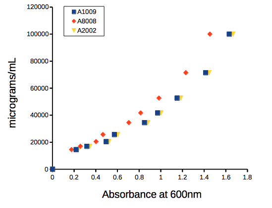
Figure 1. mg of yeast per mL of media plotted against absorbance at 600nm, OD600.
Before we estimate the equation, just take a look at how you can “eyeball” the graph and get the answer.
Question 0. If the absorbance at 600nm for an unknown sample of yeast reads 1.0, what is the approximate concentration of the sample in μg/mL?
Hint: scan the horizontal axis and stop at “1”. Trace a straight line up from “1” towards the data. When your line intersects with the data, draw a horizontal line from the intersection point to the vertical axis. Where your horizontal line intersects with the vertical axis, that’s your guesstimate for the concentration at the absorbance of “1”.
Answer. Unfortunately, it depends on which spectrophotometer you used. If it was A1009, then you would say “40,000.” If it was A8008, then you would report “50,000.”
Question 1. Did we “interpolate” or “extrapolate” to get our answer to question 0?
The relationship is curve-linear, so a semi-log10 transform is applicable (transform the concentration data). Linear equation coefficients for each of the spectrophotomers relating concentration to absorbance are given the table:
Table 2. Linear coefficients and fit statistics
| Spectrophotometer | intercept | slope | R2 |
| A1009 | 4.042 | 0.585 | 0.997 |
| A8008 | 4.069 | 0.65 | 0.995 |
| A2002 | 4.042 | 0.581 | 0.997 |
where the equation is log10(Y) = intercept + slope (X) and X is absorbance and Y is concentration of yeast. The fit statistic, R2, is called the “coefficient of determination.” R2 can range from 0 for an extremely poor fit to the data up to 1 for a perfect fit between the predicted line and the original data.
Use the equation to change your absorbance readings to estimated concentration of yeast.
An example. Let’s say you want to estimate the yeast concentration at an absorbance reading of 0.05 on the A1009 spectrophotometer. Let X = 0.05 and enter it into the equation to predict the log10 concentration (you should get 4.07125).
Don’t forget to convert the calculated concentration back to un-transformed units. For example, if the log10 Y value is 4.07125, then the inverse-log (aka antilog) can be used to convert back to the original units. Here, the inverse-log10 is 104.07125 (the answer is 11,783 μg of yeast/mL, rounded).
Example DNA calibration curve with Nanovue
Table 3. DNA Data from Dohm
| A260 nm | Concentration |
| 27.55 | 1383 |
| 26.33 | 1322 |
| 22.65 | 1124 |
| 20.35 | 1022 |
| 19.46 | 916 |
| 15.96 | 816 |
| 14.35 | 739.5 |
| 12.97 | 672.5 |
| 12.24 | 636 |
| 11.38 | 589.5 |
| 9.73 | 517 |
| 8.66 | 464 |
| 6.66 | 366 |
| 7.56 | 344.5 |
| 5.35 | 292.5 |
| 4.77 | 267 |
| 4.62 | 241.5 |
| 4.02 | 224.5 |
| 3.71 | 208.5 |
| 2.91 | 168.5 |
We could do the plotting and analysis in Google Sheets or Microsoft Excel, but nothing wrong with using mycurvefit.com (or better, use R)! Just choose the linear fit method and copy/paste the data into the table. Here’s the graph and fit statistics (Fig 2).
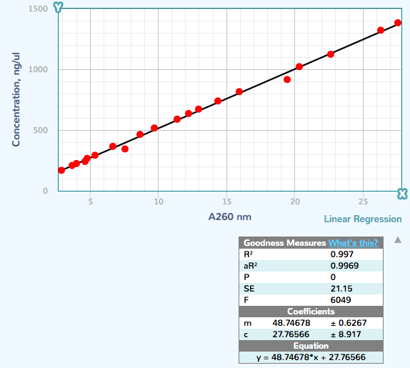
Figure 2. Screenshot results from mycurvefit.com.
The Y-intercept and the slope were 27.77 and 48.75, respectively.
References
Mohler et al (1996) Spectrophotometric quantification of tissue culture cell number in any medium. Biotechniques 21(2):260-266.
/MD