Cell counts by spectrophotometer
Cell counting is a routine and necessary task. Knowing exact cell counts ensures experimental reproducibility, keeps extractions within the chemical and physical limits of the kits we use, and lets us compare different strains or treatments. Without standardizing how many cells we start with, we cannot tell whether an observed result comes from the experimental variable or simply from starting with more or fewer cells.
There are a few standard ways to obtain cell counts, each with advantages and limitations. A hemocytometer provides exact cell concentrations (cells/mL) by direct microscopic counting, OD600 via spectrophotometer allows us to track culture density via light scattering. Spot assays measure viable cell counts (colony-forming units) through serial dilution plating. While a hemocytometer gives precise physical counts — and can assess viability if paired with a dye like Trypan blue — it is slow, tedious, and easily skewed by clumping or budding cells. Conversely, Optical density (eg, OD600) is fast and ideal for tracking real-time growth, but it cannot distinguish live cells from dead cells or debris, loses linearity at high densities, and varies with cell size or shape. Finally, spot assays directly quantify cells capable of dividing into visible colonies, though they are only semi-quantitative, sensitive to cell clumping, and require 1 to 3 days to grow.
This page describes use of optical density and the spectrophotometer for counts, provides links to excellent articles on use of hemocytometers. Spot assays are described on the next page (click here to follow link).
Approximate counts by spectrophotometer
If cells are grown in suspension, eg, bacteria, yeast, or Schneider cells, then if light is passed through the suspension, the amount of light passed through the suspension will be inversely related to the concentration of the cells in the suspension. An absorbance reading at 600 nm is used and original suspension may need to be diluted to keep within the limits of the spectrophotometer. Optical density readings between 0.1 and 0.7 are optimal — above an OD of 1.0 and 90% or more of the transmitted light is scattered, noticeable nonlinear.
This technique relies on light scattering, turbidity, not light absorption, and the Beer-Lambert law does not strictly apply to scattering in dense suspensions. Whereas absorption suggests light is absorbed by molecules within the solution, changing energy states, cells in suspended solution scatter light, which reduces detector intensity. Light scattering is proportional to cell concentration over a narrow range. True absorbance follows the Beer-Lambert law, making scattering better for microbial growth monitoring and absorbance better for molecular quantification. What is often called “absorbance” at 600 nm for cell cultures is actually “extinction,” or the sum of scattering and absorption. Typically, readings are then reported as OD600.
At low densities, a photon scatters off a single cell and misses the detector. At high densities, a photon may scatter off one cell, hit another cell, and be scattered back towards the detector. This causes the detector to receive more light than it should, resulting in a lower-than-expected OD reading and an underestimation of density.
As the culture becomes very turbid, very little light passes through to the detector. The small amount of light that is detected might be stray light rather than actual signal, causing the reading to flatten out regardless of real increases in cell concentration.
Hemocytometer Cell Counts
The hemocytometer is a specialized counting chamber that resembles a microscope slide.
A hemocytometer measures exact cell concentration (cells/mL) by loading a diluted cell suspension into a precision-etched glass chamber of known volume and counting cells under a microscope. See Wikipedia.
Hemocytometer Counter
Improved Neubauer chamber — 1 mm² large squares, standard chamber depth 0.1 mm.
Enter 10 for a 1:10 dilution. Concentrations are corrected to the original sample.
Counting grid
Click a square to select it. Press L for live cells, D for dead cells, or Backspace to undo. In Custom mode, Shift-click toggles inclusion.
Boundary rule: include cells touching top and left lines; exclude bottom and right.
Current chamber results
0
0
—
Chamber comparison
| Chamber | Squares | Live | Dead | Cells/mL | Viability |
|---|
The calculator features
- Interactive Neubauer counting grid: Select individual counting squares and record cell counts.
- Keyboard counting: Press designated keys to increment live and dead cells without looking away from the microscope.
- Multiple squares: Record counts independently for each selected square.
- Boundary rules: Display the standard inclusion/exclusion rules for cells touching grid lines.
- Viability: Calculate percentage viability when using trypan blue or methylene blue staining.
- Cell concentration: Automatically calculate cells/mL using the appropriate chamber volume and dilution factor.
- Replicate measurements: Support two chamber counts and report mean, SD, and coefficient of variation.
- Data export: Download results as CSV for analysis in R or LibreOffice Calc.
Quick Hemocytometer Protocol (Neubauer Improved)
1. Prep the Slide & Sample
- Clean & seat the coverslip: Wipe the hemocytometer and thick glass coverslip with 70% ethanol and dry with a lint-free tissue. Place the coverslip over the counting grid (moistening the outer glass shoulders slightly helps it adhere).
- Dilute & mix your culture: Yeast cultures usually need a 10-fold to 100-fold dilution so you end up with 20 to 50 cells per large square (too crowded causes counting errors; too sparse increases statistical error). If checking viability, mix 1:1 with Trypan blue or Methylene blue or other Viability dye (remembering this adds a 2× dilution factor).
- Mix thoroughly: Always mix immediately before loading because yeast settle quickly.
2. Load the Chamber
- Pipette 10 µL of your mixed suspension into the V-shaped loading notch at the edge of the coverslip.
- Let capillary action draw the liquid smoothly across the grid—do not push the plunger past the first stop or overfill the side trenches (if it overflows or traps air bubbles, clean the slide and reload).
- Let the slide sit flat for 1–2 minutes so cells settle onto the same focal plane.
3. Count Under the Microscope
- Focus on the grid lines using the 10× objective, then switch to 20× or 40× to count yeast cells clearly.
- For yeast (small cells): Count cells inside the 5 smaller squares of the central 1 mm × 1 mm grid (typically the 4 corners and the center square of the central grid, which equals 0.2 mm² total area, or 0.02 µL volume).
- Apply the boundary rule: Count cells touching the top and left border lines of each square, and ignore cells touching the bottom and right lines so you never double-count.
- Budding rule: Count a budding yeast cell as one cell unless the daughter bud is at least half the size of the mother cell.
4. Calculate Concentration (cells/mL)
Each large 1 mm × 1 mm square holds a volume of 0.1 mm³ = 10⁻⁴ mL.
If you counted the 5 sub-squares of the central grid (which represents 1/5 of the central 10⁻⁴ mL square):

If you counted all 4 large corner squares (standard for larger mammalian cells):

Example: You dilute yeast 1:10 in water, then mix 1:1 with Methylene blue (total dilution factor = 20). You count 140 live (clear) cells across the 5 central sub-squares:

Viability with dyes
Membrane-exclusion dyes — those that stain dead cells — includes
- Trypan blue: Typically a 1:1 suspension of cells in solution with the dye. Living cells actively exclude the dye from crossing the cell membrane. Dead cells absorb the dye and appear dark blue under a standard microscope, while live cells remain clear with a bright halo.
- Erythrosin B: A pink/red non-toxic dye used under a standard brightfield microscope. It works identically to Trypan blue (staining dead cells pink) and is often preferred for yeast because it gives clearer contrast and is safer to handle.
- Propidium Iodide (PI): A red-fluorescent dye that binds to DNA. Because it is membrane-impermeable, it only stains dead cells and is the gold standard for flow cytometry and fluorescence microscopy.
- SYTOX Green / DAPI (at low concentrations): Fluorescent nucleic acid stains that are excluded from live cells with intact membranes, producing a bright fluorescent signal only in dead cells.
Alternatively, some dyes enter all cells, relying on active cellular enzymes or reducing power to generate (or clear) a color or fluorescent signal. These metabolic and enzymatic dyes include:
- Methylene Blue: A brightfield dye that enters both live and dead cells. Metabolically active yeast cells possess reductase enzymes that chemically reduce the dye into a colorless form (leaving live cells clear), whereas dead cells lack this enzyme activity and remain stained dark blue.
- Fluorescein Diacetate (FDA) or Calcein-AM: Non-fluorescent molecules that pass freely into cells. Inside live cells, active esterase enzymes cleave them into bright green-fluorescent compounds, while dead cells remain dark.
- FUN-1: A yeast-specific two-color fluorescent probe. Metabolically active yeast cells process the dye into distinct, bright red cylindrical structures inside their vacuoles, whereas dead cells glow a diffuse yellow-green.
- Resazurin (Alamar Blue) and MTT/XTT: Used primarily in microplate readers rather than microscopy. Living cells chemically reduce these dyes, causing a measurable color change (eg, blue to fluorescent pink for resazurin) that indicates overall culture viability.
When to use a metabolic dye instead of an exclusion dye? Choose a metabolic dye over an exclusion dye when you need to detect early cellular damage, distinguish dormant cells from active ones, or measure live cells directly rather than just dead ones. Exclusion dyes only tell you whether a cell’s outer membrane has physically ruptured; metabolic dyes confirm that the cell’s internal machinery is actually working.
Table 1. Working Concentrations, Mixing Ratios, and Incubation Times for Common Yeast Viability Dyes.
| Dye | Typical Mixing Ratio / Dilution | Final Working Concentration | Incubation Time | Key Protocol Note |
|---|---|---|---|---|
| Trypan Blue | 1:1 (cells : 0.4% dye) | 0.2% (2 mg/mL) | 1–3 min | Count within 3–5 min; over time, the dye becomes toxic and enters live cells. |
| Methylene Blue | 1:1 (cells : 0.01%–0.1% dye) | 0.005%–0.05% | 1–5 min | Often prepared in 2% sodium citrate buffer to prevent yeast clumping and maintain optimal pH (~4.5–5.0). |
| Erythrosin B | 1:1 (cells : 0.1%–0.4% dye) | 0.05%–0.2% | 1–5 min | Less toxic than Trypan blue, giving you a longer window before live cells start absorbing dye. |
| Propidium Iodide (PI) | Spike from stock (e.g., 1:100 to 1:1,000) | 1–5 µg/mL | 5–15 min (in the dark) | Requires PBS or buffer wash first; residual media or ethanol can interfere with staining. |
| SYTOX Green | Spike from stock (e.g., 1:1,000 to 1:10,000) | 0.1–1 µM | 10–15 min (in the dark) | Very bright; dilute cells in buffer (like PBS or water) because high salt or media components quench fluorescence. |
| FDA / Calcein-AM | Spike from stock (1:100 to 1:1,000) | 1–10 µg/mL (or 1–5 µM) | 15–30 min (at room temp or 30°C) | Stock is dissolved in DMSO or acetone; keep final solvent concentration ≤1% so you don’t permeabilize live cells. |
| FUN-1 | Spike from stock (1:1,000) | 5–20 µM | 30 min (at 30°C, in the dark) | Cells must be suspended in a 2% glucose + HEPES buffer (GH solution)—without sugar, live yeast lack the ATP needed to form red vacuolar cylinders. |
| Resazurin (Alamar Blue) | 1:10 (10% of total well volume) | ~44 µM (or 10% v/v commercial reagent) | 1–4 hours (at 30°C–37°C) | Add directly to cells growing in liquid media in a 96-well plate; measure absorbance or fluorescence over time. |
Automated counters
Millipore Sceptor
Invitrogen Countess 3
Question: What is a calibration curve?
Answer: A calibration curve refers to any protocol for determining the concentration of a substance in an unknown sample by comparing the unknown to a set of standard samples of known concentration. As long as the unknown falls within the range of the data used to construct the curve (eg, scatter plot), this method yields a good estimate of the unknown value. In general, this is called interpolation, as opposed to extrapolation where the estimate would fall outside of teh range of data used to construct the calibration curve.
Example with Red Star bread yeast, growth at RT.
Three different Thermo Genesys 20S spectrophotomers were in use by Genetics class at Chaminade University. The last four digits of the model numbers are 1009, 8008, and 2002.
I started with 0.1 grams (g), or 100,000 micrograms (μg) of yeast in one milliliter (mL) media, measured absorbance of one 100 microliter (μL) aliquot plus 2.9 mL media in a cuvette one each of the three spectrophotomers, then added either 0.5 or 1 ml media (Vol1, plus Vol2 = 100 microliters to replace the Aliquot I had removed for reading), read the absorbance, etc., until I had a total of nine readings. The data are listed below in the table. “A” in front of the model number for the spectrophotometer stands for absorbance at 600 nm
Table 1. Yeast calibration data at OD600, three Thermo Genesys 20 spectrophotometers.
| μg of yeast/mL = 100K |
Total volume, mL | Vol1 | Vol2 | Aliquot | Calculated Concentration, μg/mL |
A1009 | A8008 | A2002 |
| media blank = 0 | 0 | 0 | 0.002 | 0 | 0 | |||
| 1.0 | 1.0 | 0 | 0.1 | 100000 | 1.632 | 1.454 | 1.667 | |
| 1.5 | 0.5 | 0.1 | 0.1 | 71429 | 1.414 | 1.232 | 1.446 | |
| 2.0 | 0.5 | 0.1 | 0.1 | 52632 | 1.151 | 0.984 | 1.184 | |
| 2.5 | 0.5 | 0.1 | 0.1 | 41667 | 0.971 | 0.815 | 1.002 | |
| 3.0 | 0.5 | 0.1 | 0.1 | 34483 | 0.85 | 0.706 | 0.88 | |
| 4.0 | 1.0 | 0.1 | 0.1 | 25641 | 0.572 | 0.467 | 0.603 | |
| 5.0 | 1.0 | 0.1 | 0.1 | 20408 | 0.496 | 0.403 | 0.521 | |
| 6.0 | 1.0 | 0.1 | 0.1 | 16949 | 0.318 | 0.259 | 0.346 | |
| 7.0 | 1.0 | 0.1 | 0.1 | 14493 | 0.219 | 0.177 | 0.239 |
The data are plotted in this figure 1.
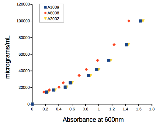
Figure 1. Scatter plot of commerical bread yeast (mg) per YPD media (mL) plotted against absorbance at 600nm, OD600.
Before we estimate the equation, just take a look at how you can “eyeball” the graph and get the answer.
Question 0. If the absorbance at 600nm for an unknown sample of yeast reads 1.0, what is the approximate concentration of the sample in  ?
Hint: scan the horizontal axis and stop at “1”. Trace a straight line up from “1” towards the data. When your line intersects with the data, draw a horizontal line from the intersection point to the vertical axis. Where your horizontal line intersects with the vertical axis, that’s your guesstimate for the concentration at the absorbance of “1”.
Answer. Unfortunately, it depends on which spectrophotometer you used. If it was A1009, then you would say “40,000.” If it was A8008, then you would report “50,000.”
Question 1. Did we “interpolate” or “extrapolate” to get our answer to question 0?
The relationship is curve-linear, so a semi-log10 transform is applicable (transform the concentration data). Linear equation coefficients for each of the spectrophotomers relating concentration to absorbance are given the table:
Table 2. Linear coefficients and fit statistics
| Spectrophotometer | intercept | slope | R2 |
| A1009 | 4.042 | 0.585 | 0.997 |
| A8008 | 4.069 | 0.65 | 0.995 |
| A2002 | 4.042 | 0.581 | 0.997 |
where the equation is  and
 is absorbance and
 is concentration of yeast. The fit statistic,
 , is called the “coefficient of determination.” can range from 0 for an extremely poor fit to the data up to 1 for a perfect fit between the predicted line and the original data.
Use the equation to change your absorbance readings to estimated concentration of yeast.
An example. Let’s say you want to estimate the yeast concentration at an absorbance reading of 0.05 on the A1009 spectrophotometer. Let  and enter it into the equation to predict the log10 concentration (you should get 4.07125).
Don’t forget to convert the calculated concentration back to un-transformed units. For example, if the  value is 4.07125, then the inverse-log (aka antilog) can be used to convert back to the original units. Here, the inverse,
 , which is 104.07125 (the answer is 11,783 μg of yeast/mL, rounded).
Example DNA calibration curve with Nanovue
Table 3. DNA Data from Dohm
| A260 nm | Concentration |
| 27.55 | 1383 |
| 26.33 | 1322 |
| 22.65 | 1124 |
| 20.35 | 1022 |
| 19.46 | 916 |
| 15.96 | 816 |
| 14.35 | 739.5 |
| 12.97 | 672.5 |
| 12.24 | 636 |
| 11.38 | 589.5 |
| 9.73 | 517 |
| 8.66 | 464 |
| 6.66 | 366 |
| 7.56 | 344.5 |
| 5.35 | 292.5 |
| 4.77 | 267 |
| 4.62 | 241.5 |
| 4.02 | 224.5 |
| 3.71 | 208.5 |
| 2.91 | 168.5 |
We could do the plotting and analysis in my Javascript plotter, Apple Numbers, LibreOffice Calc, Google Sheets or Microsoft Excel, but nothing wrong with using mycurvefit.com (or better, use R)! Just choose the linear fit method and copy/paste the data into the table. Here’s the graph and fit statistics (Fig 2).
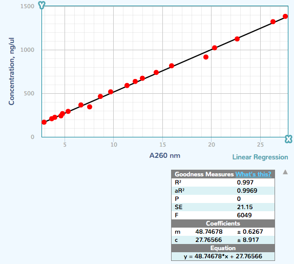
Figure 2. Screenshot results from mycurvefit.com.
The  and the slope were
27.77 and 48.75, respectively.
References
Mohler et al (1996) Spectrophotometric quantification of tissue culture cell number in any medium. Biotechniques 21(2):260-266.
/MD